Source Code: Github

Intro

In this post, I’ll show a working log of how convolution would work in CUDA, from first principles. I was initially motivated to do so after checking out nn.Conv2D module in PyTorch. For most ML programmers, the details of how this is implemented is meant to be abstracted away, but in this post, we try and bring it to light! To do so, we’ll introduce GPU programming, specifically CUDA, and how it’s useful for breaking down large 4000x4000 or more images!

Eventually, I hope to get into some optimizations I can do to make our CUDA code run even faster than it already does.

What is Convolution?

Convolution is the backbone of Convolutional Neural Networks (CNNs), vital for tasks ranging from facial recognition, self-driving cars, and even stock price prediction!

The point of convolution is to ‘combine two functions to produce a third function.’ In deep learning, this can end up being a useful feature extractor. Convolution can help detect fine grained details that allow an algorithm to make decisions without human assistance (such as the nose of a dog). In Deep Learning models such as ResNet, convolution is repeated multiple times in order to achieve optimal results.

Convolution for images has 3 properties. An input image, its corresponding filter, and the output. In a CNN, the main task is mostly devising an algorithm that can have the optimal filters in order to achieve the task at hand. A example of how convolution works can be seen here: 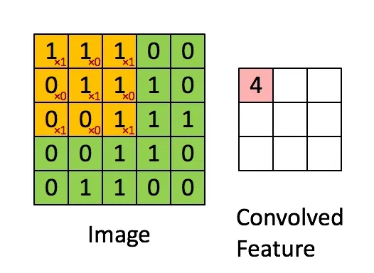Figure 1: How Convolution Works: A simple 2D Convolution Example. (Source)

As you can see, there exists an input matrix, a constant filter that multiplies its element by the current element, and then aggregating the results into one element of the resulting output. The filter then ‘slides’ over to the next matrix of elements based on something called a ‘stride.’ (In this case, set to 1). In this blog, we’ll assume a stride of 1 when programming, to make things simpler.

Why do CPUs Struggle With Convolution?

CPUs can do convolution on small images, such as the one shown above, and provide great performance. However, once image dimensions start to increase, the CPU starts to have some trouble. For a 500 x 500 image, the CPU would need to process 250,000 elements sequentially! Not to mention for a colored image, the RGB channels would require doing all steps 2 more times, yikes!

The problem is that CPUs are limited by the amount of threads that can be launched to complete a specific task, reaching a couple hundred threads executing concurrently for top of the line server CPUs. The reason for this is because CPUs are not designed to be parallelism machines. Rather, the CPU is optimized to power through any operation as fast as possible.

Simply put, the amount of threads that need to be launched for a convolution problem is too much for a CPU to handle. Given that multiple convolution passes happens in typical models, this makes for slow performance. Meanwhile, a GPU is designed to solve problems just like this!

The Power of the GPU

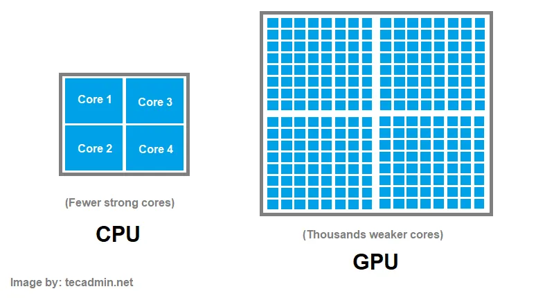Figure 2: A simplified diagram displaying CPU vs. GPU architecture. (Source)

Graphics Processing Units (GPUs) attempt to curb this problem in a unique way. A GPU is designed to have many more cores than a CPU, enabling a substantial amount of threads to be concurrently running. The tradeoff is that the many cores in a GPU are considerably weaker than that of the CPU.

GPU vendors such as NVIDIA & AMD release programming models to allow customers to write code to run on the GPU. This leads to much faster training and inference times on Deep Learning and Machine Learning models. We will be using NVIDIA’s GPU programming model, known as CUDA, to write code to run on the GPU.

How the GPU Helps Convolution

There is an inherent form of parallelism that can be exploited by convolution. Each element in the resulting output does not depend on any previous or future elements. So instead of computing each element of the output sequentially, we’ll do it at the same time!

Now, let’s get into how this can be done in CUDA.

Naive CUDA Implementation

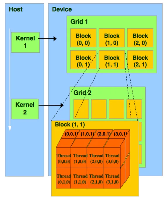Figure 3: The CUDA thread model. Source: NVIDIA

The CUDA thread model is shown in Figure 3. Code that is to be run on the GPU is a function, also known as a ‘kernel.’ The kernel launches a ‘grid’ which has a x,y,z dimension of blocks. Each block can contain threads in the x,y, and z direction.

Vector Addition

I’ll first show what a vector addition looks like in CUDA, so you get used to the syntax.

__global__ void add_vectors(double *a, double *b, double *c, int n) {
int tid = blockIdx.x * blockDim.x + threadIdx.x;
if (tid < n) {
c[tid] = a[tid] + b[tid];
}
}

As you can see, each thread has its own unique ID. The ID is a culmination of the current thread in the block, the current block in the grid, and the grid dimension, all in the X direction. The global keyword signifies that this function can be run on the GPU and can be called from CPU code. All threads run this same block of code. One array simply stores the addition of elements from two different arrays.

Convolution

Now that you know how CUDA works, it’s time to do convolution. This is a step up from normal kernels, as we have to account for threads in the Y direction, since we’re working with matrices.

Let’s start with the function parameters. We’re still going to need 3 matrices: the input image, the filter, and the resulting output. We’ll also take in the image width, filter width, filter height, and output width as additional parameters, which will be handy in calculations.

As a result, the function definition will look like so:

__global__ void convolution(int *image, int *filter, int *output,
                               int imageWidth, int filterWidth, int filterHeight, int outputWidth)

Next, it’s important to emphasize what each CUDA thread will be computing. As a reminder, each thread is supposed to compute 1 element of the output.

As a result, each time a thread launches the convolution function, we’ll need to calculate the unique thread ID. We’ll label this as the output column and the output row. Both will be a culmination of the thread ID in the X and Y direction respectively.

int outputCol = blockIdx.x * blockDim.x + threadIdx.x;
int outputRow = blockIdx.y * blockDim.y + threadIdx.y;

In convolution, in order to compute one element of the output, we must sum up the products of the filter and a specific part of the image. As a result, each thread will have a running sum that will then be placed in the output.

Now, we go deeper into what each thread should really be doing. Let’s look at the convolution gif one more time.

Each element of the output is just looping over the filter, multiplying the corresponding filter index by the current image index. As a result, each thread will also need to loop through the filter width and height.

int sum = 0;

    for (int filterRow = 0; filterRow < filterHeight; filterRow++)
    {
        for(int filterCol = 0; filterCol < filterWidth; filterCol++)
        {
            ...
        }
    }

Inside the double for loop, we need to find a way to know what corresponding element of the image we are supposed to multiply by. We don’t want threads that are meant to convolve the left side of the image accessing the right side!

As a result, we’ll derive a way to calculate the row and column of the image we’re on, which will enable us to index into the element meant to be processed.

It might help to draw out an example to see how we can derive the row and column for the image, based on the filter and output position.

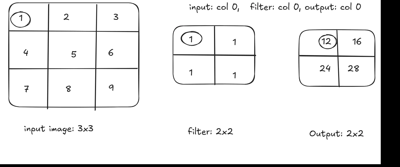Figure 4: A convolution example I made showing how the columns change as the algorithm traverses through the matrices.

Looking at figure 4, if we’re trying to derive the input image’s column from the filter and output, we can see the input image’s column is simply the sum of the filter’s column and the output’s column!

The same goes for the row calculation for the input image. The current row of the input is based on the current filter row and current output row.

We can now add to our loop that iterates over the filter:

for (int filterRow = 0; filterRow < filterHeight; filterRow++)
    {
        for(int filterCol = 0; filterCol < filterWidth; filterCol++)
        {
                int imageRow = outputRow + filterRow;
                int imageCol = outputCol + filterCol;

                ...
        }
    }

Now, we get to the core operation of convolution: taking an element of the input image, and multiplying that element by an element of the filter.

We’ll be accessing elements in a flattened 1D manner, even if all our inputs and outputs are 2D matrices. The equation to get a 1D index from a 2D matrix is:

index = currentRow * total_columns + currentColumn

The good news is, we calculated the current row of our image, we passed in the total number of columns for the image, and we already calculated the current column of our image. The same goes for our filter. The ‘filterRow’ and ‘filterCol,’ are our loop control variables. Additionally, the total number of columns in our filter is already passed in as an argument to the function.

All we have to do is multiply the two numbers based on the index and add it to our running sum, which will look like this.

for (int filterRow = 0; filterRow < filterHeight; filterRow++)
    {
        for(int filterCol = 0; filterCol < filterWidth; filterCol++)
        {
                int imageRow = outputRow + filterRow;
                int imageCol = outputCol + filterCol;

                sum += image[imageRow*imageWidth + imageCol] * filter[filterRow*filterWidth + filterCol];
        }
    }

The last thing each thread needs to do once it’s computed it’s output element is to store the running sum in the output index. Using our 1D access equation from before, and our unique outputCol and outputRow, this becomes a simple 1-liner.

    output[outputRow * outputWidth + outputCol] = sum;

There you have it! We just completed convolution in CUDA, one of the core operations behind deep learning! The full CUDA kernel altogether looks like this.

Note that in this kernel, I added outputLength as a parameter and an extra if condition. This is because we often launch more threads than needed in CUDA, in order to make sure our launches are a multiple of 32. This means threads that will be out of bounds should not be computing anything, and just skip the kernel.

__global__ void convolution(int *image, int *filter, int *output,
                            int imageWidth, int filterWidth, int filterHeight, int outputWidth, int outputLength)
{
    int outputCol = blockIdx.x * blockDim.x + threadIdx.x;
    int outputRow = blockIdx.y * blockDim.y + threadIdx.y;

    int sum = 0;
    if (outputCol < outputWidth && outputRow < outputLength)
    {
        for (int filterRow = 0; filterRow < filterHeight; filterRow++)
        {
            for (int filterCol = 0; filterCol < filterWidth; filterCol++)
            {
                int imageRow = outputRow + filterRow;
                int imageCol = outputCol + filterCol;

                sum += image[imageRow * imageWidth + imageCol] * filter[filterRow * filterWidth + filterCol];
            }
        }

        output[outputRow * outputWidth + outputCol] = sum;
    }
}
src/convolution.cu

Performance

I don’t have access to an NVIDIA GPU physically, so I access a NVIDIA GPU by using a remote cluster. In this cluster, I use an A30 GPU and a Intel Xeon Gold 6342 CPU. Needless to say, this is considerably powerful, so results will be much faster than what you may find on your own desktop GPU or laptop.

For a 4000x4000 image, a C++ CPU only implementation runs for about 1.5 seconds. Using our CUDA code, the implementation runs for about 0.5 seconds. Nice! A 3x speedup.

Disclaimer: I used the ‘time’ command in Linux to test CPU vs GPU performance. However, there are robust ways of measuring CPU vs. GPU performance not mentioned. The ‘time’ command still gives the reader a rough idea of the performance gains you see with a GPU vs. a CPU.

Work in Progress: Optimization

I plan on implementing some optimizations to make this run even faster. I’ll first try a shared memory/tiling approach before moving on to Im2Col.

Conclusion

In this post, we learned about convolution, the algorithm behind convolutional neural networks (CNNs). We learned why convolution is better suited to run on a GPU, and how to write CUDA code in order to take advantage of the paralellism provided by a GPU to do convolution. Check out the source code on Github to see the full CUDA kernels as well as my tests.